Appendix A — Interpretation of the Outputs of Statistical Tests

Here we explain how to interpret the results of the statistical tests in R, mostly in a simple way to avoid lots of confusion.

I’ve kept it very simple, but included some resources for further reading - however, these extra bits are not required reading but may help further your own understanding.

Really, we just care that you understand what the test compares and how to interpret the results of that test, while also thinking about the results in a biological context.

A.1 Chi-Square Test

The Chi-square test is used to compare observed categorical data with expected values.

It tells us if the difference between observed and expected values is due to random chance, or represents a statistically significant relationship.

So, as an example, in the UK Demographic dataset we considered if the observed number of females and males deviated from the expected number, with a null hypothesis being that the two populations should be the same.

We run the test below, and can see the output summary.

chisq.test(table(UKDemographic$Sex))


    Chi-squared test for given probabilities

data:  table(UKDemographic$Sex)
X-squared = 89.75, df = 1, p-value < 2.2e-16

We get a Chi-square value (X-squared) which is round(data_chisq[["statistic"]][["X-squared"]], digits = 2) , a degree of freedom value (df) which is 1, and a probability value (p-value) which is <2.2e-16.

Note

In the interest of keeping things simple for you, I’ve purposefully not included the full explanation of how to use the Chi-square test formula to determine the Chi-Square value - if you wish to run through a worked example, this page may be of interest to you.

The Chi-square value is used to determine significance by using the Chi-square lookup table:

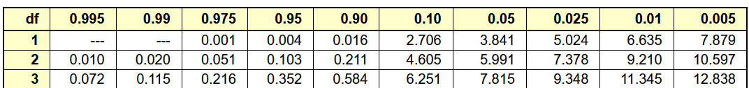
In this table, the rows are your degrees of freedom (df) and the column values are the significance value you want to check at.

To check if your chi-square value is significant, determine what your df is and then check the value in the table against your chi-square value at a given significance value.

In our test, there’s two factors in sex for this dataset, Male or Female. So since the df = n - 1, where n is the number of factors in the test, it’s simply 2 - 1. So, df = 1, so we’ll use the first rows chi-square values and compare them against our own.

The Chi-square value in our test is round(data_chisq[["statistic"]][["X-squared"]], digits = 2) , which is greater than the value in 0.05 which is 3.841. So this tells us the probability of observing the values we obtained is less than 0.05 (or p-value < 0.05). You can actually see in this case that the value is greater than any value at any p-value where df = 1, so really we could say that the p-value < 0.005 if we wanted to.

This is just giving you an example of how this is determined - the significance is already determined in the output as p-value < 2.2e-16 , so we know that this is a really significant result. Remember, if the p-value > 0.05, then we usually say this is not a significant result.

Note

If the Chi-Squared value is greater than the appropriate value in the table, the observed data is significantly different from the expected data. Therefore, there is more likely to be an association between the collected data and the variable in question.

So, based on the p-value, we could say:

The chi-squared analysis suggests that it is extremely unlikely that we would have observed as big of a difference in the ratio of males and females as expected under the null hypothesis of equal numbers. Therefore, we should be inclined to reject the null hypothesis.

Challenge yourself to frame the results in interpreting the biology behind the result.

A.2 Students T-test

The T-test is used to determine if there are significant differences between the means of two groups.

Note

Once again we’ll keep this very simple and just focus on interpretation of the output from R, but there’s some nice worked examples available online if you’re interested in seeing how the formulas work, or the underlying assumptions and different forms of the test.

So, as a nice easy example, we previously considered comparing the mean of the length of the left foot against the mean of the length of the right foot in the Me, Myself, and I dataset.

t.test(MMILabData$LengthLeftFoot, MMILabData$LengthRightFoot)


    Welch Two Sample t-test

data:  MMILabData$LengthLeftFoot and MMILabData$LengthRightFoot
t = 0.0014605, df = 1545.9, p-value = 0.9988
alternative hypothesis: true difference in means is not equal to 0
95 percent confidence interval:
 -0.2600837  0.2604713
sample estimates:
mean of x mean of y 
 24.19535  24.19516

There’s more to this but we can pick out some important bits.

The values under mean of x mean of y tell you what the mean values are of your first variable (x) and your second variable (y) - if confused about which is x and which is y, this is just the order of the variables in the test - also given in the output of data: MMILabData$LengthLeftFoot and MMILabData$LengthRightFoot .
- So, the mean of LengthLeftFoot (x) is 24.19535 and the mean of LengthRightFoot (y) is 24.19516 .
The probability of observing the difference of means is given by p-value = which in this test was ttest_results[["p.value"]] .
- Now, the p-value is > 0.05 - so this is not a significant result - and so we fail to reject the null hypothesis.
- Which indicates that the mean of the Length of the Left foot and the mean Length of the Right foot in this dataset do not significantly differ from one another.
We can see the 95 percent confidence interval: ranges from values -0.2600837 to 0.2604713.
- This just means that the length of the left foot compared to the right may vary from -0.2600837 cm to 0.2604713 cm.

And really that’s the most important outputs of the test.

So, based on the p-value we fail to reject the null hypothesis - so the means are not statistically significantly different from one another. We can see that the mean of either foot is not too dissimilar, and the confidence interval is also small as well, which supports the results of the test.

Challenge yourself to frame the results in interpreting the biology behind the result.

A.3 Linear Regression

Let’s also point out the important parts of the Linear Regression output.

Note

Once again, we’ve kept it simple, and easily interpretable. If you want a more detailed explanation, here’s one resource that gives worked context in R.

In this case, we’ll use a linear regression from the Me, Myself, and I dataset where Height is our response variable (what is changed) and Age and Sex as our explanatory variables (testing what is the effective of these on our response variable).

summary(lm(UKDemographic$Height ~ UKDemographic$Age + UKDemographic$Sex))


Call:
lm(formula = UKDemographic$Height ~ UKDemographic$Age + UKDemographic$Sex)

Residuals:
    Min      1Q  Median      3Q     Max 
-94.304  -7.147   2.635  10.473  37.902 

Coefficients:
                       Estimate Std. Error t value Pr(>|t|)    
(Intercept)           1.427e+02  3.159e-01  451.78   <2e-16 ***
UKDemographic$Age     3.312e-01  6.105e-03   54.26   <2e-16 ***
UKDemographic$SexMale 1.118e+01  2.742e-01   40.77   <2e-16 ***
---
Signif. codes:  0 '***' 0.001 '**' 0.01 '*' 0.05 '.' 0.1 ' ' 1

Residual standard error: 15.8 on 13381 degrees of freedom
Multiple R-squared:  0.2501,    Adjusted R-squared:   0.25 
F-statistic:  2231 on 2 and 13381 DF,  p-value: < 2.2e-16

Let’s focus on what’s important:

Estimate are the values for each parameter (the intercept and each level of an explanatory variable) that indicate the effect of each parameter on the response variable.
- The estimate for the intercept is the predicted value of our response variable when our continuous dependent variables are at zero, and/or for the reference level of a factor.
- The estimate for additional levels of a factor are how much we should modify the response variable for a given level of the factor.
- The estimate for a continuous explanatory variable is a measure of how much each unit of the explanatory variable modifies the response variable.
- In the context of our example test, the intercept indicates the predicted height if the Age was 0 and the Sex was “Female”.
  - You might question why it chooses “Female” over “Male” for the reference level of Sex - unless otherwise specified, the levels will be organised alphabetically, so the reference level in this case would be the first factor sorted alphabetically.
- What can we do with this information? We can use it to make a formula predicting height with these explanatory variables.
  - Height = 1.427e+02 + (Age * 3.312e-01) + (1.118e+01 if Sex = Male) cm
  - Height = 142.7 + (Age * 0.3312) + (11.18 if Sex = Male) cm
    - Note that in this second formula we’ve just removed the x10 exponent.
  - So, if we wanted to predict the height of a 52 year old Female:
    - Height = 142.7 + (52 * 0.3312) + (Sex = Female) cm
    - Height = 142.7 + 17.2224 + 0 cm
    - Height = 159. 9224 cm
Pr(>|t|) is the probability that each parameter would have the apparent impact on the response variable if the null hypothesis for each parameter was true.
Adjusted R-squared value is the proportion of the variance of our rersponse variable that is explained by the explanatory variable(s)
- It is on a scale from 0 (no predictive value) to 1 (completely predictive), but we could multiply it by 100 to convert it to the percentage of the variance of our dependent variable that is explained by the explanatory variable(s).
- In this case the adjusted R-squared was 0.25, revealing that Age and Height together account for ~ 25% of the variance in height in the UK demographic population using a simple linear model applied to the whole population.
- Sometimes when there is no real association and/or the sample size is small, we may observe a low negative adjusted R-squared value.
  - As the theoretical minimum for an R-squared value is zero, a negative adjusted R-squared value is not meaningful and is an artefact of the correction process applied to take in to account the number of independent explanatory variables incorporated into the model.
  - If ever we see such a negative adjusted R-squared value, the model p-value will almost certainly be high, and we can conclude that there is no good evidence to reject the null hypothesis.
p-value is the p-value for the overall model that provides an indication of the probability that we would have revealed an association between the response variable and the explanatory variable(s) of the magnitude observed, if the null hypothesis was correct and none of the explanatory variable(s) were truly associated with the response variable.
- In this case, the p-value observed was < 2.2e-16
- This is very low, and allows us to safely conclude that we can reject the null hypothesis and infer that at least one of our explanatory variables is providing a meaningful insight into variation in our response variable.