   Height_cm     Reflex_pathway_length_mm Mean_simple_reaction_time_mSec
 Min.   :152.5   Min.   :1170             Min.   :211.0
 1st Qu.:164.3   1st Qu.:1485             1st Qu.:261.0
 Median :169.0   Median :1570             Median :279.3
 Mean   :169.9   Mean   :1562             Mean   :283.8
 3rd Qu.:174.8   3rd Qu.:1660             3rd Qu.:299.7
 Max.   :196.0   Max.   :2025             Max.   :374.0
 Mean_choice_reaction_time_mSec Ankle_jerk_Latency_mSec Conduction_Velocity_ms
 Min.   :275.7                  Min.   :20.50           Min.   :26.40
 1st Qu.:353.5                  1st Qu.:29.44           1st Qu.:43.33
 Median :376.3                  Median :32.58           Median :47.63
 Mean   :385.5                  Mean   :32.56           Mean   :48.96
 3rd Qu.:405.3                  3rd Qu.:35.76           3rd Qu.:53.65
 Max.   :540.0                  Max.   :45.44           Max.   :79.02
 Mean_Amplitude_normal_reflex_conditions_mV     Sex
 Min.   :0.010                              Female:133
 1st Qu.:0.410                              Male  : 62
 Median :0.920
 Mean   :1.276
 3rd Qu.:1.810
Max. :4.990 6 Tutorial 2 - Scatter plots, linear regression, categorical variables (Ankle Data)
6.1 Load the Ankle Jerk Data in R
We will utilise a new dataset in R, the collection of Ankle Jerk Reflex data that you have been collecting so far: Reflex_Data_Stats.csv [this will need to be created and cleaned up so that column names are clear].
Load that dataset into R, using the 1st tutorial instructions if required.
Note
We recommend working on the same R script that you used previously, even though its a different dataset it makes it easier if all the code for functions and visualisation are on the same script, rather than multiple different locations.
The first thing you can do with a new dataset is run the summary command to understand the different variables that comprise the dataset:
Looking at the data variables being examined, how many variables are we measuring?
Looking at the the number of observations (obs.) of the data in the environment pane, how many samples are measured?
Looking at Height, is this continuous or categorical data?
Looking at Sex, is this continuous or categorical data?
Looking at Mean_simple_reaction_time_mSec, is this continuous or categorical data?
6.2 Make a Scatter plot comparing continuous variables
To generate a scatter plot between two variables so we can examine the relationship, we’ll use the tilde symbol ~
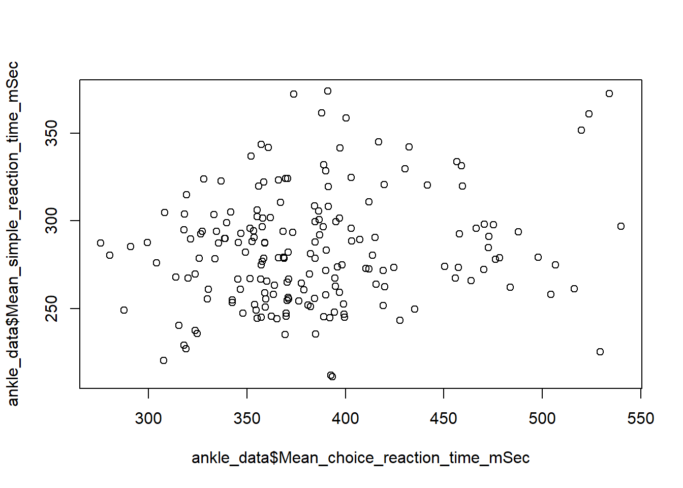
We could have just used a , between the variables and the plot would look the same.
However, we’re investigating a relationship it’s good practice to start using the ~ as in the formula for exploring a relationship we’ll typically use dependent_variable ~ Explanatory_variablewhere we are essentially asking: “how is the dependent variable affected by the explanatory variable?
E.g. what is the relationship between Mean Simple Reaction Time and Mean Choice Reaction Time?
You’ll see more of this later, but for now always use a ~ instead of a , .
What is the null hypothesis for the relationship between Simple Reaction Time and Choice Reaction Time?
The null hypothesis would be that there is no association between the Simple Reaction Time and the Choice Reaction Time.
We have also not performed the statistical test for this yet, so we could not say whether we accept or reject the null hypothesis at this point.
Note that this question relates specifically to the association between these two variables in individuals (i.e., does knowing anything about one variable provide any information about the other variable in a pair of observations from an individual)
Note that the question is asking about the association between these two variables in individuals (so does knowing the values of one variable provide information about the other variable in individuals).
The previous question for the T test was asking about comparing the means (or population averages) - so this is different from the relationship. As this is a different question, our null hypotheses will be different, so we cannot comment on the mean values between these variables with a linear regression.
To determine if there is a significant association between the two variables, we will use a regression analysis.
6.3 Perform Linear Regression
To investigate the relationship between Simple Reaction Time and Choice Reaction Time, we’ll run a linear regression analysis.
In this case, the Simple Reaction Time will be our response variable and Choice Reaction Time will be our explanatory variable:
Response_variable ~ Explanatory_variable
What we’re asking is: how is the Simple Reaction Time (Response Variable) affected by changes in the Choice Reaction Time (Explanatory Variable).
The actual function to run linear regression is simply lm, but to simplify the output we’ll run summary on the results.
Call:
lm(formula = ankle_data$Mean_simple_reaction_time_mSec ~ ankle_data$Mean_choice_reaction_time_mSec)

Residuals:
    Min      1Q  Median      3Q     Max
-74.934 -23.734  -2.096  16.810  89.896

Coefficients:
                                           Estimate Std. Error t value Pr(>|t|)
(Intercept)                               239.63387   16.71715  14.335  < 2e-16
ankle_data$Mean_choice_reaction_time_mSec   0.11454    0.04296   2.666  0.00832

(Intercept)                               ***
ankle_data$Mean_choice_reaction_time_mSec **
---
Signif. codes:  0 '***' 0.001 '**' 0.01 '*' 0.05 '.' 0.1 ' ' 1

Residual standard error: 32.04 on 193 degrees of freedom
Multiple R-squared:  0.03553,   Adjusted R-squared:  0.03053
F-statistic: 7.109 on 1 and 193 DF,  p-value: 0.008321
The output looks intense, but it’s easily understandable once you know what to look for.
For now, let’s add use the output of the lm to add a regression line (or line of best fit) to our scatter plot!
By running the below code, you should have a regression line added to your scatter plot:
Warning
If this hasn’t worked, make sure that you have:
Made the plot and it shows in the plot panel
You have used the
~instead of the,in the plot function
Now, let’s go back to the output of the summary(lm) and see if we can determine some answers from it.
How much of the variation in Simple Reaction Time can be predicted by Choice Reaction Time?
Determining how much of the variation in Simple Reaction Time can be predicted by knowing the Choice Reaction Time is determined by the Adjusted R-squared value - so 0.0305 .
If we multiplied this answer by 100, we obtain the percentage variation of the explanatory variable affecting the response variable.
E.g. if R-squared was 0.01, then 1% of the variability in Simple Reaction Time can be explained by its relationship with Choice Reaction Time - which isn’t a lot!
What is the probability that we would have observed an association of this magnitude if the null hypothesis were correct, and we had collected a random sample of the population? You can just copy the answer directly from the output.
The probability that we would have observed an association of this magnitude if the null hypothesis were correct, and we had collected a random sample of the population, is simply given by the p-value - which we can see is 0.008321 so we’ll use that as an answer.
Should we reject the null hypothesis?
Given that this p-value is less than 0.05 we would be inclined to reject the null hypothesis - suggesting that it is extremely unlikely that we would observe the association between these two variables if the null was correct and our sample was unbiased with respect to this parameter. Therefore, we can be highly confident in rejecting the null hypothesis.
What is the null hypothesis for the intercept value for the association between Simple Reaction Time and Choice Reaction Time? (e.g, what null hypothesis can we think of for the value of the Simple Reaction Time, when the Choice Reaction Time is set to 0). Choose 1 correct answer.
If we’re looking at the intercept, then the x-axis value (Choice Reaction Time) is set to 0, and we’re asking what the value in our y-axis (Simple Reaction Time) would be.
If the Choice Reaction Time at the intercept is set to the value of 0, the null hypothesis for the Simple Reaction Time would be 0 as well - we’re essentially saying that they won’t differ from each other under a null hypothesis.
What is the predicted intercept in the association test for Simple Reaction Time and Choice Reaction Time?
The actual predicted intercept in the association test for Simple Reaction Time and Choice Reaction Time is returned in the Coefficients section, looking at the (Intercept) and the Estimate section - which is 239.633866. So, when the Choice Reaction Time is set to 0, the predicted Simple Reaction Time is 239.633866.
As a note, the value below the (Intercept) is ankle_data$Mean_choice_reaction_time_mSec - the values here indicate the predicted increase in Mean_simple_reaction_time_mSec with every unit increase of Mean Choice Reaction Time.
So, for every 1 millisecond increase in Mean Choice Reaction Time, there’s a predicted increase of 0.114541 in the Simple Reaction Time - essentially telling us that if someone’s Choice Reaction Time increases, so to will the Simple Reaction Time.
You could then create a formula to predict Simple Reaction Time knowing the Choice Reaction Time, using these intercept values.
Mean Simple Reaction Time = 239.63387 + 0.11454 * Mean Choice Reaction Time
So if someone’s Choice Reaction Time was 385:
Mean Simple Reaction Time = 239.63387 + 0.11454 * 385
Mean Simple Reaction Time = 239.63387 + 44.0979
Mean Simple Reaction Time = 283.7322
The only thing to remember, is that the accuracy of this formula also depends on the predictive power of the test - so if the adjusted R-squared value is low, then it will be less accurate.
What is the probability that we would have observed an intercept of this magnitude if the null hypothesis were correct?
The probability that we would have observed an intercept of this magnitude is given in the same Coefficients section, at the end Pr(>|t|). We can see this is < 2e-16
Should we reject the null hypothesis regarding the intercept? I.e., are we confident in saying that the Simple Reaction would not be 0 if the Choice Reaction time is 0?
In this case, yes it makes sense to reject the null hypothesis - the choice reaction time is never going to be 0, as its impossible to be - so we would always expect that the intercept for Simple Reaction Time would never be 0.
Instead, it makes more sense to focus on the relationship between these two variables rather than their intercept.
Note
If you want a case where considering the intercept is interesting, in the previous data we used we had the length of left foot and the length of the right foot.
If you ran a linear regression with this data, looking at the relationship between the two variables with the left foot being the response variable, you would find the intercept of the length of the left foot to be slightly above 1 (e.g. when the length of the right foot is set to 0, the length of the left foot is bigger!).
This seems like a weird result! Surely we would 1:1 relationship, in that both feet should be of similar sizes!
Well, if we made a scatter plot of left against right foot length, we would see some outliers in the data were people have (hopefully) made an error in the measurement and given themselves a difference of 10cm in foot length! This is an example of a type 1 error!
6.4 Using a categorical predictor
Now we’ll use what we’ve learned so far and apply this to new variables to investigate, so far we’ve investigated continuous data but now we’ll look at some categorical data to see how this differs.
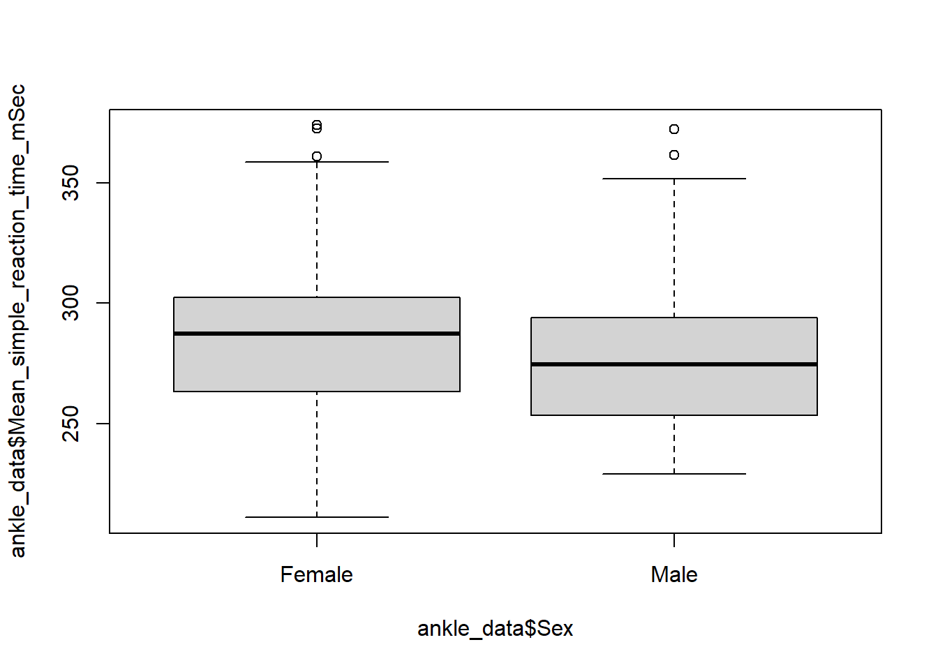
Generate a boxplot of the Simple Reaction Time dependent on Sex.
6.4.1 T-test of continuous variable dependent on categorical variables
Perform a T test to determine if the mean values of Simple Reaction Time differ dependent on Sex.
    Welch Two Sample t-test

data:  ankle_data$Mean_simple_reaction_time_mSec by ankle_data$Sex
t = 1.5757, df = 125.32, p-value = 0.1176
alternative hypothesis: true difference in means between group Female and group Male is not equal to 0
95 percent confidence interval:
 -1.971172 17.372070
sample estimates:
mean in group Female   mean in group Male
            286.2327             278.5323
Why did we use a ~ here, when we used a , to separate variables in the previous T test we did?
You might want to run ?t.test to investigate the arguments further to pick the correct answers.
There’s no such thing as “statistical matchmaking mode” - it’s total nonsense.
The other options are correct, and can be found in the ?t.test help panel.
Basically, because Sex is categorical (Male or Female in this case) and we’re investigating if Simple Reaction Time is dependent on Sex, we need to use the tilde. This is just a requirement of the function, as read in the help panel.
Previously, we could just use a comma because we were looking at comparing the means of two continuous variables.
Now try to answer the questions about the output of the t.test:
What is the difference in Mean Simple Reaction Time between males and females?
The mean of the male simple reaction time is 278.5323 and the mean of the female simple reaction time is 286.2327.
Simply subtract the higher number from the other.
You can use R as a calculator, so just get the two values and write:
value1 - value2
What are the 95% confidence intervals for the difference in Mean Simple Reaction Time between males and females?
to
The 95% confidence intervals for the difference in Mean Simple Reaction Time between males and females is returned in the output under 95 percent confidence interval.
What does the confidence interval values tell us about the difference in reaction times between Females and Males?
Female reaction time is .
The confidence intervals tell us how the range in which the variables we’re investigating differ in their mean values. If both the values were negative, it tells us that the first level (Females) of our variable is on average always less than the second (Males). E.g. if it was - 10 -5 then the reaction time of Females would generally be lower than that of males by a range of 10 to 5 mSecs.
As the range in our output of the T-test goes from minus to positive, we can see that there is a wider spread of values - so in this case there’s likely no real difference between the two, some females have a shorter reaction time, some have a longer reaction time, compared to males.
We can visualise this better with the boxplot comparing males and females - to see they are not too dissimilar.
Note
The reason why it chooses Females first is a quirk of factors - it chooses the levels of a factor alphabetically, so it goes Females first then Males. To see this, you could run levels(ankle_data$Sex). If you wanted to reorder the levels to Males then Females, you could do so by running levels(ankle_data$Sex) = c("Males", "Females").
6.5 Linear regression with categorical predictor
Now, perform a regression analysis to investigate the relationship between Simple Reaction Time and Sex.
Call:
lm(formula = ankle_data$Mean_simple_reaction_time_mSec ~ ankle_data$Sex)

Residuals:
    Min      1Q  Median      3Q     Max
-75.233 -23.882  -3.532  15.932  93.798

Coefficients:
                   Estimate Std. Error t value Pr(>|t|)
(Intercept)         286.233      2.812 101.805   <2e-16 ***
ankle_data$SexMale   -7.700      4.986  -1.544    0.124
---
Signif. codes:  0 '***' 0.001 '**' 0.01 '*' 0.05 '.' 0.1 ' ' 1

Residual standard error: 32.42 on 193 degrees of freedom
Multiple R-squared:  0.01221,   Adjusted R-squared:  0.007089
F-statistic: 2.385 on 1 and 193 DF,  p-value: 0.1241
How much of the variation in Simple Reaction Time can be predicted by Sex? Give this answer as a percentage, and round to 1 decimal place.
So for variation being predicted, we look at the adjusted R-squared value. We now want to express this as a percentage, so multiply the adjusted R-squared value by 100.
What is the probability that we would have observed an association of this magnitude if the null hypothesis were correct?
2.2e-16
Let’s look at the p-value under adjusted R-squared, as we’re looking at the association.
What is the intercept for the regression analysis between Simple Reaction Time and Sex?
We’re looking at the intercept again - with a categorical predictor this time, Sex. The actual intercept for the regression analysis is given by the Estimate value.
With a categorical predictor in a regression analysis, the intercept is set to the first level in the categorical predictor - which in this case is Female as we assigned no set level, so it just works alphabetically.
So, we can see underneath the Estimate that if they are Male, there’s an decrease in the value (e.g. the simple reaction time is predicted to decrease).
Use the results of the regression analysis to produce a formula for predicting Simple Reaction Time dependent on Sex.
Length of the left foot = (- if male) cm
As explained in the solution above, with a categorical predictor the intercept is set to the first level in which in this case is Female.
So, we can see underneath the Estimate that if they are Male, there’s a decrease of -7.700449 .
As this is a categorical predictor, unlike the previous T-test in Tutorial 1 where we were looking at a continuous predictor (LengthLeftFoot), this is a one-time decrease if the Sex is Male. If you remember, with a continuous predictor, it was a unit increase/decrease every time there was an increase/decrease in the predictor as well - have a look back to understand the difference.
What is the likely cause and effect relationship between Simple Reaction Time and Sex?
The results tell us that Females will have a Mean Simple Reaction Time of round(lm_results2[["coefficients"]][1], digits = 6) cm, while males have a Mean Simple Reaction Time of round(lm_results2[["coefficients"]][1], digits = 6)- abs(round(lm_results2[["coefficients"]][2], digits = 6)) cm.
The effect of sex on average foot length does not seem significant, (p-value > 0.05), and based on the adjusted R-squared we can see that sex only accounts for round(lm_results2[["adj.r.squared"]]*100, digit = 1) of the variation in the length of the left foot - it accounts for a minuscule amount of variation in the Simple Reaction Time.
If we wanted to justify our answer, what could we say?
If we base our answer on the results of the statistical tests we’ve performed, then the the p-value is insignificant and we fail to reject the null hypothesis testing the association.
Added to this, the adjusted R-squared, which tells us how much of the variance in Simple Reaction Time is accounted for by Sex, explains less than 1% of the variance.
Therefore, biological sex seems to have no associated with the results of the Mean Simple Reaction Time.
In the case of explaining these results, it may be of interest to consider if there could be limitations of the dataset that affect the results of statistical tests - for example, could the dataset be skewed to a particular Sex and therefore if we added more of the under-represented Sex would we have obtained a more interesting result? Or perhaps we have quite a small sample group that doesn’t represent a general population (e.g., these are all measurements taken by students at a University in Scotland, will these be representative of the whole of the UK, or particular age demographics?). Or, as these are measurements taken by students who are likely performing these sorts of tests for the first time - could there be errors in measurements that are affecting the results? This would be an example of a type 2 error in the test we ran above, as we are accepting a false null hypothesis.
6.6 Using height as response variable
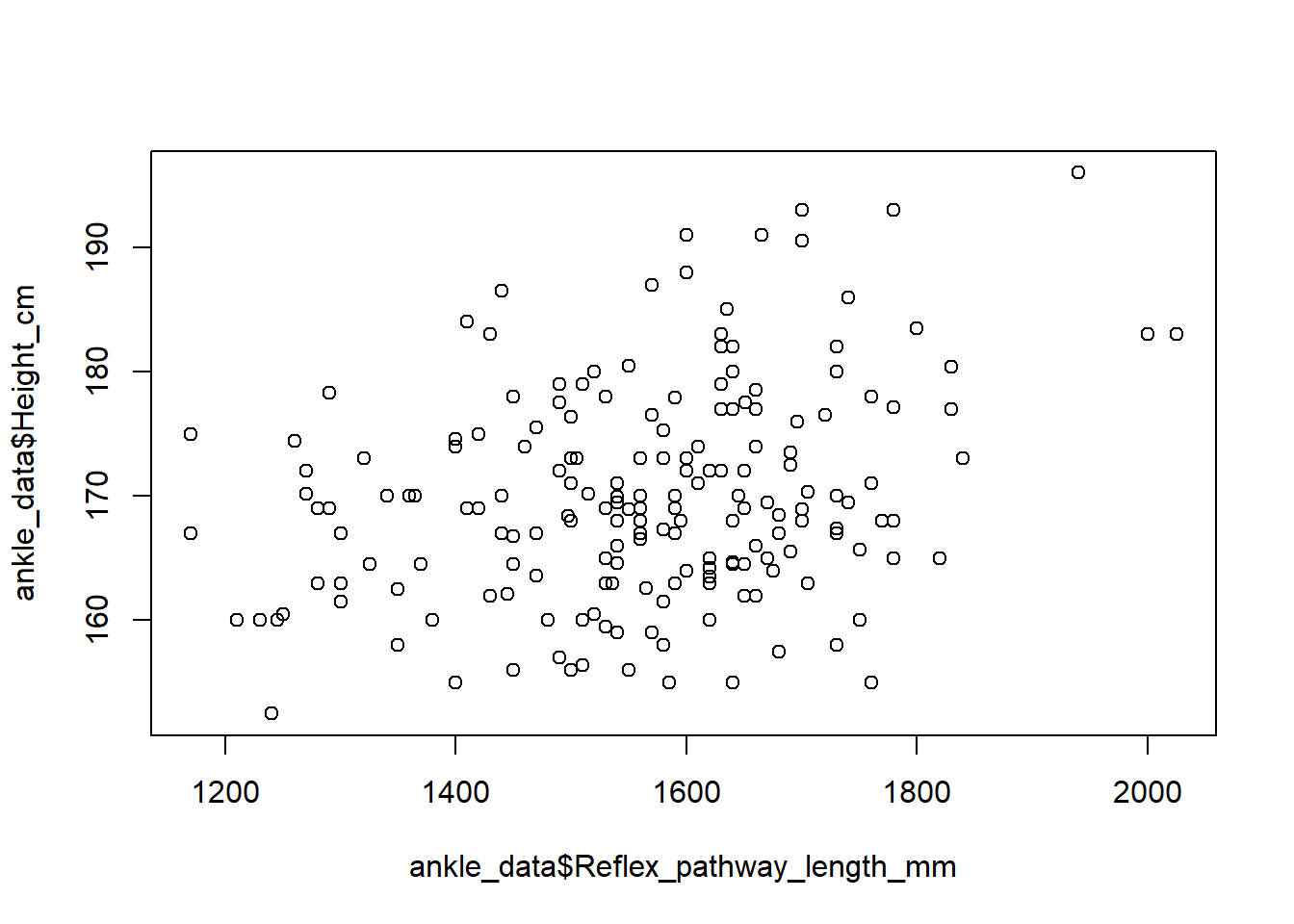
Let’s now look at the relationship between Height and dependent on Reflex Pathway Length.
Can you make a scatterplot of the two?
Now, perform a regression analysis for Height dependent on the Reflex Pathway Length.
Call:
lm(formula = ankle_data$Height_cm ~ ankle_data$Reflex_pathway_length_mm)

Residuals:
    Min      1Q  Median      3Q     Max
-17.969  -5.838  -1.025   5.344  20.958

Coefficients:
                                     Estimate Std. Error t value Pr(>|t|)
(Intercept)                         1.458e+02  5.938e+00  24.550  < 2e-16 ***
ankle_data$Reflex_pathway_length_mm 1.545e-02  3.784e-03   4.083 6.51e-05 ***
---
Signif. codes:  0 '***' 0.001 '**' 0.01 '*' 0.05 '.' 0.1 ' ' 1

Residual standard error: 8.095 on 193 degrees of freedom
Multiple R-squared:  0.07951,   Adjusted R-squared:  0.07474
F-statistic: 16.67 on 1 and 193 DF,  p-value: 6.506e-05
Add the regression line to the scatterplot.
Now answer the questions about the regression analysis.
Note that to answer the questions about Ankle Jerk Latency, you’ll need to do another regression analysis (Height as response variable, Ankle Jerk Latency as predictor variable).
How much of the variation in Height can be predicted by Reflex Pathway Length? Express this answer as a percentage, and round nearest whole number.
Remember, variation in response variable is given by adjusted R-squared. Express as a percentage by multiplying by 100.
Perform another regression analysis for Height dependent on Ankle Jerk Latency. Is Reflex Pathway Length or Ankle Jerk Latency more powerful in predicting Height?
The Reflex Pathway Length predicts ~ of the variation in height.
Ankle Jerk Latency predicts ~ of the variation in height.
Therefore, Ankle Jerk Latency is Reflex Pathway Length in predicting Height.
Use the variation given by adjusted R-squared to answer this question. Remember, the higher the variation explained the more this accurately predicts the response variable.
Are these meaningful results?
Now, one thing to note is that in both cases the intercept values and the result of the tests are significant. What we can say with this is that there is a relationship between the explanatory variables and the response variable (and that in the case of our intercepts that the response variable differs from 0 when the explanatory variables are set to 0). However, the low adjusted r-squared tells us that the model explains only a small fraction of the total variance in the data. If it accounts for a low amount of variance, then it’s not good at making accurate predictions of the response variable from the explanatory variable.
There could be some reasons for why the result comes out like this: perhaps it is just a poor way of explaining the variance; perhaps there are other variables that we haven’t investigated that better account for the variance; perhaps there are issues in the data, for instance perhaps data measurements are inaccurate because it is the first time some students are taking these measurements; perhaps if we added more samples then the result would be more accurate (think about the demographic that provided the data for this dataset, is it truly representative of a given population? Is there a bias towards a certain group e.g. in terms of Sex?).
Given that we expect to see some sort of relationship between Height & Reflex Pathway Length (longer legs mean longer Reflex Pathway Lengths) there could very well be some mistakes in the student collected data, or maybe we should have measured legs instead of Height!
6.7 Performing regression analysis with multiple variables
Perform a regression analysis of Height dependent on Reflex Pathway Length and Ankle Jerk Latency.
When we use multiple explanatory variables, we have to change the formula to include them in the design.
So, something like: lm(response_variable ~ explanatory_variable_1 + explanatory_variable_2)
That way, both explanatory variables are accounted for in the relationship with the response variable.
So, try to think about how to write the function so we can see the relationship of Height (response variable) with Sex and Ankle Jerk Latency (explanatory variables).
How much of the variation in Height can be predicted by Reflex Pathway Length and Ankle Jerk Latency combined? Express this answer as a percentage, and round to nearest whole number.
How confident are we that Reflex Pathway Length and Ankle Jerk Latency are independent predictors of Height? For the values below, round to 2 decimal places instead of rounding to whole number as previously.
From the previous regression analysis, we found that Reflex Pathway Length predicts ~ of the variation in height.
Likewise, Ankle Jerk Latency was found to predict ~ of the variation in height.
If the two explanatory variables are truly independent, then the result of combining the two variables in the regression analysis would result in an additive percentage variation being explained (the variation explained in both tests could be added together, resulting in additive effect). If this was the case, then using both variables in the model would result in an additive percentage variation explained of .
However, we found that when we included both explanatory variables in the model, then they only accounted for of the variance in Height. This is than the additive amount we calculated above.
Therefore, Reflex Pathway Length and Ankle Jerk Latency completely independent.
Since the variance explained by both explanatory variables is also either explanatory variable alone, and the p-values for both explanatory variables are 0.05, then they are .
What is the formula derived from the regression analysis for predicting Height based on Reflex Pathway Length and Ankle Jerk Latency?
Height = + ( * Reflex Pathway Length mm) + ( * Ankle Jerk Latency mSec) cm
6.8 Assessment Tasks
Just FYI me, here’s the things that I feel like could be tested and are most applicable to what suggestions the team put forward:
Heights relationship with reaction time (not significant)
Latency related to height (we actually ended up checking this in the tutorial)
Reflex pathway length affected by height (also checked this in the tutorial)
Male v female populations (chi-sq test, I’ve simulated data to make it biased towards women)
Simple reaction time v Choice reaction time (easy T test, sig result)
Get them to run a multiple linear regression (they pick, and have to interpret)